Friday, July 17, 2015

Taking cricketr for a spin - Part 1

“Curiouser and curiouser!” cried Alice
“The time has come,” the walrus said, “to talk of many things: Of shoes and ships - and sealing wax - of cabbages and kings”
“Begin at the beginning,”the King said, very gravely,“and go on till you come to the end: then stop.”
“And what is the use of a book,” thought Alice, “without pictures or conversation?”
            Excerpts from Alice in Wonderland by Lewis Carroll

Introduction

This post is a continuation of my previous post "Introducing cricketr! A R package to analyze the performances of cricketers." In this post I take my package cricketr for a spin. For this analysis I focus on the Indian batting legends
- Sachin Tendulkar (Master Blaster)
- Rahul Dravid (The Will)
- Sourav Ganguly ( The Dada Prince)
- Sunil Gavaskar (Little Master)
This post is also hosted on RPubs - cricketr-1
library(devtools)
install_github("tvganesh/cricketr")
library(cricketr)

Box Histogram Plot

This plot shows a combined boxplot of the Runs ranges and a histogram of the Runs Frequency The plot below indicate the Tendulkar’s average is the highest. He is followed by Dravid, Gavaskar and then Ganguly
batsmanPerfBoxHist("./tendulkar.csv","Sachin Tendulkar")
tkps-boxhist-1

batsmanPerfBoxHist("./dravid.csv","Rahul Dravid")
tkps-boxhist-2

batsmanPerfBoxHist("./ganguly.csv","Sourav Ganguly")
tkps-boxhist-3

batsmanPerfBoxHist("./gavaskar.csv","Sunil Gavaskar")
 
tkps-boxhist-4

Relative Mean Strike Rate

In this first plot I plot the Mean Strike Rate of the batsmen. Tendulkar leads in the Mean Strike Rate for each runs in the range 100- 180. Ganguly has a very good Mean Strike Rate for runs range 40 -80
frames <- span=""> list("./tendulkar.csv","./dravid.csv","ganguly.csv","gavaskar.csv")
names <- span=""> list("Tendulkar","Dravid","Ganguly","Gavaskar")
relativeBatsmanSR(frames,names)
plot-1-1

Relative Runs Frequency Percentage

The plot below show the percentage contribution in each 10 runs bucket over the entire career.The percentage Runs Frequency is fairly close but Gavaskar seems to lead most of the way
frames <- span=""> list("./tendulkar.csv","./dravid.csv","ganguly.csv","gavaskar.csv")
names <- span=""> list("Tendulkar","Dravid","Ganguly","Gavaskar")
relativeRunsFreqPerf(frames,names)
plot-2-1

Moving Average of runs over career

The moving average for the 4 batsmen indicate the following - Tendulkar and Ganguly’s career has a downward trend and their retirement didn’t come too soon - Dravid and Gavaskar’s career definitely shows an upswing. They probably had a year or two left.
par(mfrow=c(2,2))
par(mar=c(4,4,2,2))
batsmanMovingAverage("./tendulkar.csv","Tendulkar")
batsmanMovingAverage("./dravid.csv","Dravid")
batsmanMovingAverage("./ganguly.csv","Ganguly")
batsmanMovingAverage("./gavaskar.csv","Gavaskar")
tdsg-ma-1
dev.off()
## null device 
##           1

Runs forecast

The forecast for the batsman is shown below. The plots indicate that only Tendulkar seemed to maintain a consistency over the period while the rest seem to score less than their forecasted runs in the last 10% of the career
par(mfrow=c(2,2))
par(mar=c(4,4,2,2))
batsmanPerfForecast("./tendulkar.csv","Sachin Tendulkar")
batsmanPerfForecast("./dravid.csv","Rahul Dravid")
batsmanPerfForecast("./ganguly.csv","Sourav Ganguly")
batsmanPerfForecast("./gavaskar.csv","Sunil Gavaskar")
tdsg-perf-1
dev.off()
## null device 
##           1

Check for batsman in-form/out-of-form

The following snippet checks whether the batsman is in-inform or ouyt-of-form during the last 10% innings of the career. This is done by choosing the null hypothesis (h0) to indicate that the batsmen are in-form. Ha is the alternative hypothesis that they are not-in-form. The population is based on the 1st 90% of career runs. The last 10% is taken as the sample and a check is made on the lower tail to see if the sample mean is less than 95% confidence interval. If this difference is >0.05 then the batsman is considered out-of-form.
The computation show that Tendulkar was out-of-form while the other’s weren’t. While Dravid and Gavaskar’s moving average do show an upward trend the surprise is Ganguly. This could be that Ganguly was able to keep his average in the last 10% to with the 95$ confidence interval. It has to be noted that Ganguly’s average was much lower than Tendulkar
checkBatsmanInForm("./tendulkar.csv","Tendulkar")
## *******************************************************************************************
## 
## Population size: 294  Mean of population: 50.48 
## Sample size: 33  Mean of sample: 32.42 SD of sample: 29.8 
## 
## Null hypothesis H0 : Tendulkar 's sample average is within 95% confidence interval 
##         of population average
## Alternative hypothesis Ha : Tendulkar 's sample average is below the 95% confidence
##         interval of population average
## 
## [1] "Tendulkar 's Form Status: Out-of-Form because the p value: 0.000713  is less than alpha=  0.05"
## *******************************************************************************************
checkBatsmanInForm("./dravid.csv","Dravid")
## *******************************************************************************************
## 
## Population size: 256  Mean of population: 46.98 
## Sample size: 29  Mean of sample: 43.48 SD of sample: 40.89 
## 
## Null hypothesis H0 : Dravid 's sample average is within 95% confidence interval 
##         of population average
## Alternative hypothesis Ha : Dravid 's sample average is below the 95% confidence
##         interval of population average
## 
## [1] "Dravid 's Form Status: In-Form because the p value: 0.324138  is greater than alpha=  0.05"
## *******************************************************************************************
checkBatsmanInForm("./ganguly.csv","Ganguly")
## *******************************************************************************************
## 
## Population size: 169  Mean of population: 38.94 
## Sample size: 19  Mean of sample: 33.21 SD of sample: 32.97 
## 
## Null hypothesis H0 : Ganguly 's sample average is within 95% confidence interval 
##         of population average
## Alternative hypothesis Ha : Ganguly 's sample average is below the 95% confidence
##         interval of population average
## 
## [1] "Ganguly 's Form Status: In-Form because the p value: 0.229006  is greater than alpha=  0.05"
## *******************************************************************************************
checkBatsmanInForm("./gavaskar.csv","Gavaskar")
## *******************************************************************************************
## 
## Population size: 125  Mean of population: 44.67 
## Sample size: 14  Mean of sample: 57.86 SD of sample: 58.55 
## 
## Null hypothesis H0 : Gavaskar 's sample average is within 95% confidence interval 
##         of population average
## Alternative hypothesis Ha : Gavaskar 's sample average is below the 95% confidence
##         interval of population average
## 
## [1] "Gavaskar 's Form Status: In-Form because the p value: 0.793276  is greater than alpha=  0.05"
## *******************************************************************************************
dev.off()
## null device 
##           1

3D plot of Runs vs Balls Faced and Minutes at Crease

The plot is a scatter plot of Runs vs Balls faced and Minutes at Crease. A prediction plane is fitted
par(mfrow=c(1,2))
par(mar=c(4,4,2,2))
battingPerf3d("./tendulkar.csv","Tendulkar")
battingPerf3d("./dravid.csv","Dravid")
plot-3-1
par(mfrow=c(1,2))
par(mar=c(4,4,2,2))
battingPerf3d("./ganguly.csv","Ganguly")
battingPerf3d("./gavaskar.csv","Gavaskar")
plot-4-1
dev.off()
## null device 
##           1

Predicting Runs given Balls Faced and Minutes at Crease

A multi-variate regression plane is fitted between Runs and Balls faced +Minutes at crease.
BF <- span=""> seq( 10, 400,length=15)
Mins <- span=""> seq(30,600,length=15)
newDF <- span=""> data.frame(BF,Mins)
tendulkar <- span=""> batsmanRunsPredict("./tendulkar.csv","Tendulkar",newdataframe=newDF)
dravid <- span=""> batsmanRunsPredict("./dravid.csv","Dravid",newdataframe=newDF)
ganguly <- span=""> batsmanRunsPredict("./ganguly.csv","Ganguly",newdataframe=newDF)
gavaskar <- span=""> batsmanRunsPredict("./gavaskar.csv","Gavaskar",newdataframe=newDF)
The fitted model is then used to predict the runs that the batsmen will score for a given Balls faced and Minutes at crease. It can be seen Tendulkar has a much higher Runs scored than all of the others.
Tendulkar is followed by Ganguly who we saw earlier had a very good strike rate. However it must be noted that Dravid and Gavaskar have a better average.
batsmen <- span="">cbind(round(tendulkar$Runs),round(dravid$Runs),round(ganguly$Runs),round(gavaskar$Runs))
colnames(batsmen) <- span=""> c("Tendulkar","Dravid","Ganguly","Gavaskar")
newDF <- span=""> data.frame(round(newDF$BF),round(newDF$Mins))
colnames(newDF) <- span=""> c("BallsFaced","MinsAtCrease")
predictedRuns <- span=""> cbind(newDF,batsmen)
predictedRuns
##    BallsFaced MinsAtCrease Tendulkar Dravid Ganguly Gavaskar
## 1          10           30         7      1       7        4
## 2          38           71        23     14      21       17
## 3          66          111        39     27      35       30
## 4          94          152        54     40      50       43
## 5         121          193        70     54      64       56
## 6         149          234        86     67      78       69
## 7         177          274       102     80      93       82
## 8         205          315       118     94     107       95
## 9         233          356       134    107     121      108
## 10        261          396       150    120     136      121
## 11        289          437       165    134     150      134
## 12        316          478       181    147     165      147
## 13        344          519       197    160     179      160
## 14        372          559       213    173     193      173
## 15        400          600       229    187     208      186

Contribution to matches won and lost

par(mfrow=c(2,2))
par(mar=c(4,4,2,2))
batsmanContributionWonLost(35320,"Tendulkar")
batsmanContributionWonLost(28114,"Dravid")
batsmanContributionWonLost(28779,"Ganguly")
batsmanContributionWonLost(28794,"Gavaskar")
tdgg-1

Home and overseas performance

From the plot below Tendulkar and Dravid have a lot more matches both home and abroad and their performance has good both at home and overseas. Tendulkar has the best performance home and abroad and is consistent all across. Dravid is also cossistent at all venues. Gavaskar played fewer matches than Tendulkar & Dravid. The range of runs at home is higher than overseas, however the average is consistent both at home and abroad. Finally we have Ganguly.
par(mfrow=c(2,2))
par(mar=c(4,4,2,2))
batsmanPerfHomeAway(35320,"Tendulkar")
batsmanPerfHomeAway(28114,"Dravid")
batsmanPerfHomeAway(28779,"Ganguly")
batsmanPerfHomeAway(28794,"Gavaskar")
tdgg-ha-1

Average runs at ground and against opposition

Tendulkar has above 50 runs average against Sri Lanka, Bangladesh, West Indies and Zimbabwe. The performance against Australia and England average very close to 50. Sydney, Port Elizabeth, Bloemfontein, Collombo are great huntings grounds for Tendulkar
par(mfrow=c(1,2))
par(mar=c(4,4,2,2))
batsmanAvgRunsGround("./tendulkar.csv","Tendulkar")
batsmanAvgRunsOpposition("./tendulkar.csv","Tendulkar")
avgrg-1-1

dev.off()
## null device 
##           1
Dravid plundered runs at Adelaide, Georgetown, Oval, Hamiltom etc. Dravid has above average against England, Bangaldesh, New Zealand, Pakistan, West Indies and Zimbabwe
par(mfrow=c(1,2))
par(mar=c(4,4,2,2))
batsmanAvgRunsGround("./dravid.csv","Dravid")
batsmanAvgRunsOpposition("./dravid.csv","Dravid")
avgrg-2-1

dev.off()
## null device 
##           1
Ganguly has good performance at the Oval, Rawalpindi, Johannesburg and Kandy. Ganguly averages 50 runs against England and Bangladesh.
par(mfrow=c(1,2))
par(mar=c(4,4,2,2))
batsmanAvgRunsGround("./ganguly.csv","Ganguly")
batsmanAvgRunsOpposition("./ganguly.csv","Ganguly")
avgrg-3-1

dev.off()
## null device 
##           1
The Oval, Sydney, Perth, Melbourne, Brisbane, Manchester are happy hunting grounds for Gavaskar. Gavaskar averages around 50 runs Australia, Pakistan, Sri Lanka, West Indies.
par(mfrow=c(1,2))
par(mar=c(4,4,2,2))
batsmanAvgRunsGround("./gavaskar.csv","Gavaskar")
batsmanAvgRunsOpposition("./gavaskar.csv","Gavaskar")
avgrg-4-1

dev.off()
## null device 
##           1

Key findings

Here are some key conclusions
  1. Tendulkar has the highest average among the 4. He is followed by Dravid, Gavaskar and Ganguly.
  2. Tendulkar’s predicted performance for a given number of Balls Faced and Minutes at Crease is superior to the rest
  3. Dravid averages above 50 against 6 countries
  4. West Indies and Australia are Gavaskar’s favorite batting grounds
  5. Ganguly has a very good Mean Strike Rate for the range 40-80 and Tendulkar from 100-180
  6. In home and overseas performance, Tendulkar is the best. Dravid and Gavaskar also have good performance overseas.
  7. Dravid and Gavaskar probably retired a year or two earlier while Tendulkar and Ganguly’s time was clearly up

Final thoughts

Tendulkar is clearly the greatest batsman India has produced as he leads in almost all aspects of batting - number of centuries, strike rate, predicted runs and home and overseas performance. Dravid follows Tendulkar with 48 centuries, consistent performance home and overseas and a career that was still green. Gavaskar has fewer matches than rest but his performance overseas is very good in those helmetless times. Finally we have Ganguly.
Dravid and Gavaskar had a few more years of great batting while Tendulkar and Ganguly’s career was on a decline.
Note:It is really not fair to include Gavaskar in the analysis as he played in a different era when helmets were not used, even against the fiery pace of Thomson, Lillee, Roberts, Holding etc. In addition Gavaskar did not play against some of the newer countries like Bangladesh and Zimbabwe where he could have amassed runs. Yet I wanted to include him and his performance is clearly excellent
Also see my other posts in R
  1. A peek into literacy in India: Statistical Learning with R
  2. A crime map of India in R - Crimes against women
  3. Analyzing cricket’s batting legends - Through the mirage with R
  4. Masters of Spin: Unraveling the web with R
  5. Mirror, mirror . the best batsman of them all?
You may also like
  1. A crime map of India in R: Crimes against women
  2. What’s up Watson? Using IBM Watson’s QAAPI with Bluemix, NodeExpress - Part 1
  3. Bend it like Bluemix, MongoDB with autoscaling - Part 2
  4. Informed choices through Machine Learning : Analyzing Kohli, Tendulkar and Dravid
  5. Thinking Web Scale (TWS-3): Map-Reduce - Bring compute to data
  6. Deblurring with OpenCV:Weiner filter reloaded

Introducing cricketr! : An R package to analyze performances of cricketers

Yet all experience is an arch wherethro’
Gleams that untravell’d world whose margin fades
For ever and forever when I move.
How dull it is to pause, to make an end,
To rust unburnish’d, not to shine in use!

Ulysses by Alfred Tennyson

Introduction

This is an initial post in which I introduce a cricketing package ‘cricketr’ which I have created. This package was a natural culmination to my earlier posts on cricket and my completing 9 modules of Data Science Specialization, from John Hopkins University at Coursera. The thought of creating this package struck me some time back, and I have finally been able to bring this to fruition.
So here it is. My R package ‘cricketr!!!’
This package uses the statistics info available in ESPN Cricinfo Statsguru. The current version of this package only uses data from test cricket. I plan to develop functionality for One-day and Twenty20 cricket later.
You should be able to install the package from GitHub and use  many of the functions available in the package. Please be mindful of  ESPN Cricinfo Terms of Use
(Note: This page is also hosted as a GitHub page at cricketr and also at RPubs as cricketr: A R package for analyzing performances of cricketers
You can download this analysis as a PDF file from Introducing cricketr

 The cricketr package

The cricketr package has several functions that perform several different analyses on both batsman and bowlers. The package has functions that plot percentage frequency runs or wickets, runs likelihood for a batsman, relative run/strike rates of batsman and relative performance/economy rate for bowlers are available.
Other interesting functions include batting performance moving average, forecast and a function to check whether the batsman/bowler is in in-form or out-of-form.
The data for a particular player can be obtained with the getPlayerData() function from the package. To do this you will need to go to ESPN CricInfo Player and type in the name of the player for e.g Ricky Ponting, Sachin Tendulkar etc. This will bring up a page which have the profile number for the player e.g. for Sachin Tendulkar this would be http://www.espncricinfo.com/india/content/player/35320.html. Hence, Sachin’s profile is 35320. This can be used to get the data for Tendulkar as shown below
The cricketr package can be installed from GitHub with
library(devtools)
install_github("tvganesh/cricketr")
library(cricketr)
tendulkar <- span=""> getPlayerData(35320,dir="..",file="tendulkar.csv",type="batting",homeOrAway=c(1,2),
                           result=c(1,2,4))
Important Note This needs to be done only once for a player. This function stores the player’s data in a CSV file (for e.g. tendulkar.csv as above) which can then be reused for all other functions. Once we have the data for the players many analyses can be done. This post will use the stored CSV file obtained with a prior getPlayerData for all subsequent analyses

Sachin Tendulkar’s performance - Basic Analyses

The 3 plots below provide the following for Tendulkar
  1. Frequency percentage of runs in each run range over the whole career
  2. Mean Strike Rate for runs scored in the given range
  3. A histogram of runs frequency percentages in runs ranges
par(mfrow=c(1,3))
par(mar=c(4,4,2,2))
batsmanRunsFreqPerf("./tendulkar.csv","Sachin Tendulkar")
batsmanMeanStrikeRate("./tendulkar.csv","Sachin Tendulkar")
batsmanRunsRanges("./tendulkar.csv","Sachin Tendulkar")
tendulkar-batting-1
dev.off()
## null device 
##           1

More analyses

par(mfrow=c(1,3))
par(mar=c(4,4,2,2))
batsman4s("./tendulkar.csv","Tendulkar")
batsman6s("./tendulkar.csv","Tendulkar")
batsmanDismissals("./tendulkar.csv","Tendulkar")
tendulkar-4s6sout-1
 

3D scatter plot and prediction plane

The plots below show the 3D scatter plot of Sachin’s Runs versus Balls Faced and Minutes at crease. A linear regression model is then fitted between Runs and Balls Faced + Minutes at crease
battingPerf3d("./tendulkar.csv","Sachin Tendulkar")
tendulkar-3d-1

Average runs at different venues

The plot below gives the average runs scored by Tendulkar at different grounds. The plot also displays the number of innings at each ground as a label at x-axis. It can be seen Tendulkar did great in Colombo (SSC), Melbourne ifor matches overseas and Mumbai, Mohali and Bangalore at home
batsmanAvgRunsGround("./tendulkar.csv","Sachin Tendulkar")
tendulkar-avggrd-1

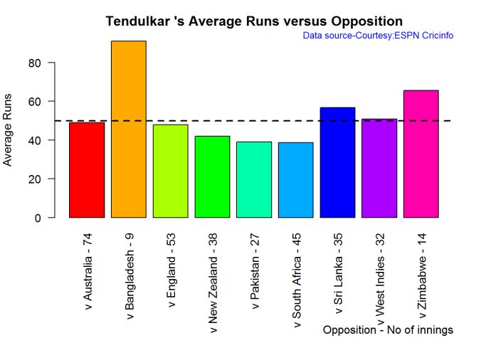
Average runs against different opposing teams

This plot computes the average runs scored by Tendulkar against different countries. The x-axis also gives the number of innings against each team
batsmanAvgRunsOpposition("./tendulkar.csv","Tendulkar")
tendulkar-avgopn-1

Highest Runs Likelihood

The plot below shows the Runs Likelihood for a batsman. For this the performance of Sachin is plotted as a 3D scatter plot with Runs versus Balls Faced + Minutes at crease using. K-Means. The centroids of 3 clusters are computed and plotted. In this plot. Sachin Tendulkar’s highest tendencies are computed and plotted using K-Means
batsmanRunsLikelihood("./tendulkar.csv","Sachin Tendulkar")
tendulkar-kmeans-1
## Summary of  Sachin Tendulkar 's runs scoring likelihood
## **************************************************
## 
## There is a 16.51 % likelihood that Sachin Tendulkar  will make  139 Runs in  251 balls over 353  Minutes 
## There is a 58.41 % likelihood that Sachin Tendulkar  will make  16 Runs in  31 balls over  44  Minutes 
## There is a 25.08 % likelihood that Sachin Tendulkar  will make  66 Runs in  122 balls over 167  Minutes

A look at the Top 4 batsman - Tendulkar, Kallis, Ponting and Sangakkara

The batsmen with the most hundreds in test cricket are
  1. Sachin Tendulkar :Average:53.78,100’s - 51, 50’s - 68
  2. Jacques Kallis : Average: 55.47, 100’s - 45, 50’s - 58
  3. Ricky Ponting : Average: 51.85, 100’s - 41 , 50’s - 62
  4. Kumara Sangakarra: Average: 58.04 ,100’s - 38 , 50’s - 52
in that order.
The following plots take a closer at their performances. The box plots show the mean (red line) and median (blue line). The two ends of the boxplot display the 25th and 75th percentile.

Box Histogram Plot

This plot shows a combined boxplot of the Runs ranges and a histogram of the Runs Frequency. The calculated Mean differ from the stated means possibly because of data cleaning. Also not sure how the means were arrived at ESPN Cricinfo for e.g. when considering not out..
batsmanPerfBoxHist("./tendulkar.csv","Sachin Tendulkar")
tkps-boxhist-1
batsmanPerfBoxHist("./kallis.csv","Jacques Kallis")
tkps-boxhist-2
batsmanPerfBoxHist("./ponting.csv","Ricky Ponting")
tkps-boxhist-3
batsmanPerfBoxHist("./sangakkara.csv","K Sangakkara")
tkps-boxhist-4

Contribution to won and lost matches

The plot below shows the contribution of Tendulkar, Kallis, Ponting and Sangakarra in matches won and lost. The plots show the range of runs scored as a boxplot (25th & 75th percentile) and the mean scored. The total matches won and lost are also printed in the plot.
All the players have scored more in the matches they won than the matches they lost. Ricky Ponting is the only batsman who seems to have more matches won to his credit than others. This could also be because he was a member of strong Australian team
par(mfrow=c(2,2))
par(mar=c(4,4,2,2))
batsmanContributionWonLost("35320","Sachin Tendulkar")
batsmanContributionWonLost("45789","Jacques Kallis")
batsmanContributionWonLost("7133","Ricky Ponting")
batsmanContributionWonLost("50710","K Sangakarra")
tkps-wonlost-1
dev.off()
## null device 
##           1

Performance at home and overseas

From the plot below it can be seen
Tendulkar has more matches overseas than at home and his performance is consistent in all venues at home or abroad. Ponting has lesser innings than Tendulkar and has an equally good performance at home and overseas.Kallis and Sangakkara’s performance abroad is lower than the performance at home.
par(mfrow=c(2,2))
par(mar=c(4,4,2,2))
batsmanPerfHomeAway("35320","Tendulkar")
batsmanPerfHomeAway("45789","Kallis")
batsmanPerfHomeAway("7133","Ponting")
batsmanPerfHomeAway("50710","Sangakarra")
tkps-homeaway-1
dev.off()
## null device 
##           1
 

Relative Mean Strike Rate plot

The plot below compares the Mean Strike Rate of the batsman for each of the runs ranges of 10 and plots them. The plot indicate the following Range 0 - 50 Runs - Ponting leads followed by Tendulkar Range 50 -100 Runs - Ponting followed by Sangakkara Range 100 - 150 - Ponting and then Tendulkar
frames <- span=""> list("./tendulkar.csv","./kallis.csv","ponting.csv","sangakkara.csv")
names <- span=""> list("Tendulkar","Kallis","Ponting","Sangakkara")
relativeBatsmanSR(frames,names)
tkps-relSR-1

Relative Runs Frequency plot

The plot below gives the relative Runs Frequency Percetages for each 10 run bucket. The plot below show
Sangakkara leads followed by Ponting
frames <- span=""> list("./tendulkar.csv","./kallis.csv","ponting.csv","sangakkara.csv")
names <- span=""> list("Tendulkar","Kallis","Ponting","Sangakkara")
relativeRunsFreqPerf(frames,names)
tkps-relRunFreq-1

Moving Average of runs in career

Take a look at the Moving Average across the career of the Top 4. Clearly . Kallis and Sangakkara have a few more years of great batting ahead. They seem to average on 50. . Tendulkar and Ponting definitely show a slump in the later years
par(mfrow=c(2,2))
par(mar=c(4,4,2,2))
batsmanMovingAverage("./tendulkar.csv","Sachin Tendulkar")
batsmanMovingAverage("./kallis.csv","Jacques Kallis")
batsmanMovingAverage("./ponting.csv","Ricky Ponting")
batsmanMovingAverage("./sangakkara.csv","K Sangakkara")
tkps-ma-1
dev.off()
## null device 
##           1

Future Runs forecast

Here are plots that forecast how the batsman will perform in future. In this case 90% of the career runs trend is uses as the training set. the remaining 10% is the test set.
A Holt-Winters forecating model is used to forecast future performance based on the 90% training set. The forecated runs trend is plotted. The test set is also plotted to see how close the forecast and the actual matches
Take a look at the runs forecasted for the batsman below.
  • Tendulkar’s forecasted performance seems to tally with his actual performance with an average of 50
  • Kallis the forecasted runs are higher than the actual runs he scored
  • Ponting seems to have a good run in the future
  • Sangakkara has a decent run in the future averaging 50 runs
par(mfrow=c(2,2))
par(mar=c(4,4,2,2))
batsmanPerfForecast("./tendulkar.csv","Sachin Tendulkar")
batsmanPerfForecast("./kallis.csv","Jacques Kallis")
batsmanPerfForecast("./ponting.csv","Ricky Ponting")
batsmanPerfForecast("./sangakkara.csv","K Sangakkara")
tkps-perffcst-1
dev.off()
## null device 
##           1

Check Batsman In-Form or Out-of-Form

The below computation uses Null Hypothesis testing and p-value to determine if the batsman is in-form or out-of-form. For this 90% of the career runs is chosen as the population and the mean computed. The last 10% is chosen to be the sample set and the sample Mean and the sample Standard Deviation are caculated.
The Null Hypothesis (H0) assumes that the batsman continues to stay in-form where the sample mean is within 95% confidence interval of population mean The Alternative (Ha) assumes that the batsman is out of form the sample mean is beyond the 95% confidence interval of the population mean.
A significance value of 0.05 is chosen and p-value us computed If p-value >= .05 - Batsman In-Form If p-value < 0.05 - Batsman Out-of-Form
Note Ideally the p-value should be done for a population that follows the Normal Distribution. But the runs population is usually left skewed. So some correction may be needed. I will revisit this later
This is done for the Top 4 batsman
checkBatsmanInForm("./tendulkar.csv","Sachin Tendulkar")
## *******************************************************************************************
## 
## Population size: 294  Mean of population: 50.48 
## Sample size: 33  Mean of sample: 32.42 SD of sample: 29.8 
## 
## Null hypothesis H0 : Sachin Tendulkar 's sample average is within 95% confidence interval 
##         of population average
## Alternative hypothesis Ha : Sachin Tendulkar 's sample average is below the 95% confidence
##         interval of population average
## 
## [1] "Sachin Tendulkar 's Form Status: Out-of-Form because the p value: 0.000713  is less than alpha=  0.05"
## *******************************************************************************************
checkBatsmanInForm("./kallis.csv","Jacques Kallis")
## *******************************************************************************************
## 
## Population size: 240  Mean of population: 47.5 
## Sample size: 27  Mean of sample: 47.11 SD of sample: 59.19 
## 
## Null hypothesis H0 : Jacques Kallis 's sample average is within 95% confidence interval 
##         of population average
## Alternative hypothesis Ha : Jacques Kallis 's sample average is below the 95% confidence
##         interval of population average
## 
## [1] "Jacques Kallis 's Form Status: In-Form because the p value: 0.48647  is greater than alpha=  0.05"
## *******************************************************************************************
checkBatsmanInForm("./ponting.csv","Ricky Ponting")
## *******************************************************************************************
## 
## Population size: 251  Mean of population: 47.5 
## Sample size: 28  Mean of sample: 36.25 SD of sample: 48.11 
## 
## Null hypothesis H0 : Ricky Ponting 's sample average is within 95% confidence interval 
##         of population average
## Alternative hypothesis Ha : Ricky Ponting 's sample average is below the 95% confidence
##         interval of population average
## 
## [1] "Ricky Ponting 's Form Status: In-Form because the p value: 0.113115  is greater than alpha=  0.05"
## *******************************************************************************************
checkBatsmanInForm("./sangakkara.csv","K Sangakkara")
## *******************************************************************************************
## 
## Population size: 193  Mean of population: 51.92 
## Sample size: 22  Mean of sample: 71.73 SD of sample: 82.87 
## 
## Null hypothesis H0 : K Sangakkara 's sample average is within 95% confidence interval 
##         of population average
## Alternative hypothesis Ha : K Sangakkara 's sample average is below the 95% confidence
##         interval of population average
## 
## [1] "K Sangakkara 's Form Status: In-Form because the p value: 0.862862  is greater than alpha=  0.05"
## *******************************************************************************************

3D plot of Runs vs Balls Faced and Minutes at Crease

The plot is a scatter plot of Runs vs Balls faced and Minutes at Crease. A prediction plane is fitted
par(mfrow=c(1,2))
par(mar=c(4,4,2,2))
battingPerf3d("./tendulkar.csv","Tendulkar")
battingPerf3d("./kallis.csv","Kallis")
plot-3-1par(mfrow=c(1,2))
par(mar=c(4,4,2,2))
battingPerf3d("./ponting.csv","Ponting")
battingPerf3d("./sangakkara.csv","Sangakkara")
plot-4-1dev.off()
## null device 
##           1

Predicting Runs given Balls Faced and Minutes at Crease

A multi-variate regression plane is fitted between Runs and Balls faced +Minutes at crease. A sample sequence of Balls Faced(BF) and Minutes at crease (Mins) is setup as shown below. The fitted model is used to predict the runs for these values
BF <- span=""> seq( 10, 400,length=15)
Mins <- span=""> seq(30,600,length=15)
newDF <- span=""> data.frame(BF,Mins)
tendulkar <- span=""> batsmanRunsPredict("./tendulkar.csv","Tendulkar",newdataframe=newDF)
kallis <- span=""> batsmanRunsPredict("./kallis.csv","Kallis",newdataframe=newDF)
ponting <- span=""> batsmanRunsPredict("./ponting.csv","Ponting",newdataframe=newDF)
sangakkara <- span=""> batsmanRunsPredict("./sangakkara.csv","Sangakkara",newdataframe=newDF)
The fitted model is then used to predict the runs that the batsmen will score for a given Balls faced and Minutes at crease. It can be seen Ponting has the will score the highest for a given Balls Faced and Minutes at crease.
Ponting is followed by Tendulkar who has Sangakkara close on his heels and finally we have Kallis. This is intuitive as we have already seen that Ponting has a highest strike rate.
batsmen <- span="">cbind(round(tendulkar$Runs),round(kallis$Runs),round(ponting$Runs),round(sangakkara$Runs))
colnames(batsmen) <- span=""> c("Tendulkar","Kallis","Ponting","Sangakkara")
newDF <- span=""> data.frame(round(newDF$BF),round(newDF$Mins))
colnames(newDF) <- span=""> c("BallsFaced","MinsAtCrease")
predictedRuns <- span=""> cbind(newDF,batsmen)
predictedRuns
##    BallsFaced MinsAtCrease Tendulkar Kallis Ponting Sangakkara
## 1          10           30         7      6       9          2
## 2          38           71        23     20      25         18
## 3          66          111        39     34      42         34
## 4          94          152        54     48      59         50
## 5         121          193        70     62      76         66
## 6         149          234        86     76      93         82
## 7         177          274       102     90     110         98
## 8         205          315       118    104     127        114
## 9         233          356       134    118     144        130
## 10        261          396       150    132     161        146
## 11        289          437       165    146     178        162
## 12        316          478       181    159     194        178
## 13        344          519       197    173     211        194
## 14        372          559       213    187     228        210
## 15        400          600       229    201     245        226

Analysis of Top 3 wicket takers

The top 3 wicket takes in test history are
1. M Muralitharan:Wickets: 800, Average = 22.72, Economy Rate - 2.47
2. Shane Warne: Wickets: 708, Average = 25.41, Economy Rate - 2.65
3. Anil Kumble: Wickets: 619, Average = 29.65, Economy Rate - 2.69
How do Anil Kumble, Shane Warne and M Muralitharan compare with one another with respect to wickets taken and the Economy Rate. The next set of plots compute and plot precisely these analyses.

Wicket Frequency Plot

This plot below computes the percentage frequency of number of wickets taken for e.g 1 wicket x%, 2 wickets y% etc and plots them as a continuous line
par(mfrow=c(1,3))
par(mar=c(4,4,2,2))
bowlerWktsFreqPercent("./kumble.csv","Anil Kumble")
bowlerWktsFreqPercent("./warne.csv","Shane Warne")
bowlerWktsFreqPercent("./murali.csv","M Muralitharan")
relBowlFP-1
dev.off()
## null device 
##           1

Wickets Runs plot

par(mfrow=c(1,3))
par(mar=c(4,4,2,2))
bowlerWktsRunsPlot("./kumble.csv","Kumble")
bowlerWktsRunsPlot("./warne.csv","Warne")
bowlerWktsRunsPlot("./murali.csv","Muralitharan")
wktsrun-1
dev.off()
## null device 
##           1

Average wickets at different venues

The plot gives the average wickets taken by Muralitharan at different venues. Muralitharan has taken an average of 8 and 6 wickets at Oval & Wellington respectively in 2 different innings. His best performances are at Kandy and Colombo (SSC)
bowlerAvgWktsGround("./murali.csv","Muralitharan")
avgWktshrg-1

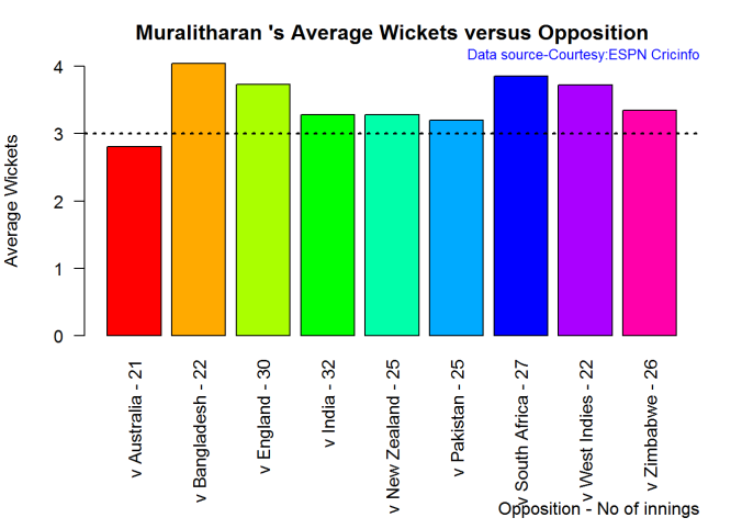
Average wickets against different opposition

The plot gives the average wickets taken by Muralitharan against different countries. The x-axis also includes the number of innings against each team
bowlerAvgWktsOpposition("./murali.csv","Muralitharan")
avgWktoppn-1

Relative Wickets Frequency Percentage

The Relative Wickets Percentage plot shows that M Muralitharan has a large percentage of wickets in the 3-8 wicket range
frames <- span=""> list("./kumble.csv","./murali.csv","warne.csv")
names <- span=""> list("Anil KUmble","M Muralitharan","Shane Warne")
relativeBowlingPerf(frames,names)
relBowlPerf-1

Relative Economy Rate against wickets taken

Clearly from the plot below it can be seen that Muralitharan has the best Economy Rate among the three
frames <- span=""> list("./kumble.csv","./murali.csv","warne.csv")
names <- span=""> list("Anil KUmble","M Muralitharan","Shane Warne")
relativeBowlingER(frames,names)
relBowlER-1

Wickets taken moving average

From th eplot below it can be see 1. Shane Warne’s performance at the time of his retirement was still at a peak of 3 wickets 2. M Muralitharan seems to have become ineffective over time with his peak years being 2004-2006 3. Anil Kumble also seems to slump down and become less effective.
par(mfrow=c(1,3))
par(mar=c(4,4,2,2))
bowlerMovingAverage("./kumble.csv","Anil Kumble")
bowlerMovingAverage("./warne.csv","Shane Warne")
bowlerMovingAverage("./murali.csv","M Muralitharan")
tkps-bowlma-1
dev.off()
## null device 
##           1

Future Wickets forecast

Here are plots that forecast how the bowler will perform in future. In this case 90% of the career wickets trend is used as the training set. the remaining 10% is the test set.
A Holt-Winters forecating model is used to forecast future performance based on the 90% training set. The forecated wickets trend is plotted. The test set is also plotted to see how close the forecast and the actual matches
Take a look at the wickets forecasted for the bowlers below. - Shane Warne and Muralitharan have a fairly consistent forecast - Kumble forecast shows a small dip
par(mfrow=c(1,3))
par(mar=c(4,4,2,2))
bowlerPerfForecast("./kumble.csv","Anil Kumble")
bowlerPerfForecast("./warne.csv","Shane Warne")
bowlerPerfForecast("./murali.csv","M Muralitharan")
kwm-perffcst-1
dev.off()
## null device 
##           1

Contribution to matches won and lost

The plot below is extremely interesting
1. Kumble wickets range from 2 to 4 wickets in matches wons with a mean of 3
2. Warne wickets in won matches range from 1 to 4 with more matches won. Clearly there are other bowlers contributing to the wins, possibly the pacers
3. Muralitharan wickets range in winning matches is more than the other 2 and ranges ranges 3 to 5 and clearly had a hand (pun unintended) in Sri Lanka’s wins
par(mfrow=c(1,3))
par(mar=c(4,4,2,2))
bowlerContributionWonLost(30176,"Anil Kumble")
bowlerContributionWonLost(8166,"Shane Warne")
bowlerContributionWonLost(49636,"M Muralitharan")
kwm-wl-1
dev.off()
## null device 
##           1

Performance home and overseas

From the plot below it can be seen that Kumble & Warne have played more matches overseas than Muralitharan. Both Kumble and Warne show an average of 2 wickers overseas,  Murali on the other hand has an average of 2.5 wickets overseas but a slightly less number of matches than Kumble & Warne
par(mfrow=c(1,3))
par(mar=c(4,4,2,2))
bowlerPerfHomeAway(30176,"Kumble")
bowlerPerfHomeAway(8166,"Warne")
bowlerPerfHomeAway(49636,"Murali")

kwm-ha-1
dev.off()
## null device 
##           1
 

Check for bowler in-form/out-of-form

The below computation uses Null Hypothesis testing and p-value to determine if the bowler is in-form or out-of-form. For this 90% of the career wickets is chosen as the population and the mean computed. The last 10% is chosen to be the sample set and the sample Mean and the sample Standard Deviation are caculated.
The Null Hypothesis (H0) assumes that the bowler continues to stay in-form where the sample mean is within 95% confidence interval of population mean The Alternative (Ha) assumes that the bowler is out of form the sample mean is beyond the 95% confidence interval of the population mean.
A significance value of 0.05 is chosen and p-value us computed If p-value >= .05 - Batsman In-Form If p-value < 0.05 - Batsman Out-of-Form
Note Ideally the p-value should be done for a population that follows the Normal Distribution. But the runs population is usually left skewed. So some correction may be needed. I will revisit this later
Note: The check for the form status of the bowlers indicate 1. That both Kumble and Muralitharan were out of form. This also shows in the moving average plot 2. Warne is still in great form and could have continued for a few more years. Too bad we didn’t see the magic later
checkBowlerInForm("./kumble.csv","Anil Kumble")
## *******************************************************************************************
## 
## Population size: 212  Mean of population: 2.69 
## Sample size: 24  Mean of sample: 2.04 SD of sample: 1.55 
## 
## Null hypothesis H0 : Anil Kumble 's sample average is within 95% confidence interval 
##         of population average
## Alternative hypothesis Ha : Anil Kumble 's sample average is below the 95% confidence
##         interval of population average
## 
## [1] "Anil Kumble 's Form Status: Out-of-Form because the p value: 0.02549  is less than alpha=  0.05"
## *******************************************************************************************
checkBowlerInForm("./warne.csv","Shane Warne")
## *******************************************************************************************
## 
## Population size: 240  Mean of population: 2.55 
## Sample size: 27  Mean of sample: 2.56 SD of sample: 1.8 
## 
## Null hypothesis H0 : Shane Warne 's sample average is within 95% confidence interval 
##         of population average
## Alternative hypothesis Ha : Shane Warne 's sample average is below the 95% confidence
##         interval of population average
## 
## [1] "Shane Warne 's Form Status: In-Form because the p value: 0.511409  is greater than alpha=  0.05"
## *******************************************************************************************
checkBowlerInForm("./murali.csv","M Muralitharan")
## *******************************************************************************************
## 
## Population size: 207  Mean of population: 3.55 
## Sample size: 23  Mean of sample: 2.87 SD of sample: 1.74 
## 
## Null hypothesis H0 : M Muralitharan 's sample average is within 95% confidence interval 
##         of population average
## Alternative hypothesis Ha : M Muralitharan 's sample average is below the 95% confidence
##         interval of population average
## 
## [1] "M Muralitharan 's Form Status: Out-of-Form because the p value: 0.036828  is less than alpha=  0.05"
## *******************************************************************************************
dev.off()
## null device 
##           1

Key Findings

The plots above capture some of the capabilities and features of my cricketr package. Feel free to install the package and try it out. Please do keep in mind ESPN Cricinfo’s Terms of Use.
Here are the main findings from the analysis above

Analysis of Top 4 batsman

The analysis of the Top 4 test batsman Tendulkar, Kallis, Ponting and Sangakkara show the folliwing
  1. Sangakkara has the highest average, followed by Tendulkar, Kallis and then Ponting.
  2. Ponting has the highest strike rate followed by Tendulkar,Sangakkara and then Kallis
  3. The predicted runs for a given Balls faced and Minutes at crease is highest for Ponting, followed by Tendulkar, Sangakkara and Kallis
  4. The moving average for Tendulkar and Ponting shows a downward trend while Kallis and Sangakkara retired too soon
  5. Tendulkar was out of form about the time of retirement while the rest were in-form. But this result has to be taken along with the moving average plot. Ponting was clearly on the way out.
  6. The home and overseas performance indicate that Tendulkar is the clear leader. He has the highest number of matches played overseas and his performance has been consistent. He is followed by Ponting, Kallis and finally Sangakkara

Analysis of Top 3 legs spinners

The analysis of Anil Kumble, Shane Warne and M Muralitharan show the following
  1. Muralitharan has the highest wickets and best economy rate followed by Warne and Kumble
  2. Muralitharan has higher wickets frequency percentage between 3 to 8 wickets
  3. Muralitharan has the best Economy Rate for wickets between 2 to 7
  4. The moving average plot shows that the time was up for Kumble and Muralitharan but Warne had a few years ahead
  5. The check for form status shows that Muralitharan and Kumble time was over while Warne still in great form
  6. Kumble’s has more matches abroad than the other 2, yet Kumble averages of 3 wickets at home and 2 wickets overseas liek Warne . Murali has played few matches but has an average of 4 wickets at home and 3 wickets overseas.

Final thoughts

Here are my final thoughts

Batting

Among the 4 batsman Tendulkar, Kallis, Ponting and Sangakkara the clear leader is Tendulkar for the following reasons
  1. Tendulkar has the highest test centuries and runs of all time.Tendulkar’s average is 2nd to Sangakkara, Tendulkar’s predicted runs for a given Balls faced and Minutes at Crease is 2nd and is behind Ponting. Also Tendulkar’s performance at home and overseas are consistent throughtout despite the fact that he has a highest number of overseas matches
  2. Ponting takes the 2nd spot with the 2nd highest number of centuries, 1st in Strike Rate and 2nd in home and away performance.
  3. The 3rd spot goes to Sangakkara, with the highest average, 3rd highest number of centuries, reasonable run frequency percentage in different run ranges. However he has a fewer number of matches overseas and his performance overseas is significantly lower than at home
  4. Kallis has the 2nd highest number of centuries but his performance overseas and strike rate are behind others
  5. Finally Kallis and Sangakkara had a few good years of batting still left in them (pity they retired!) while Tendulkar and Ponting’s time was up

Bowling

Muralitharan leads the way followed closely by Warne and finally Kumble. The reasons are
  1. Muralitharan has the highest number of test wickets with the best Wickets percentage and the best Economy Rate. Murali on average gas taken 4 wickets at home and 3 wickets overseas
  2. Warne follows Murali in the highest wickets taken, however Warne has less matches overseas than Murali and average 3 wickets home and 2 wickets overseas
  3. Kumble has the 3rd highest wickets, with 3 wickets on an average at home and 2 wickets overseas. However Kumble has played more matches overseas than the other two. In that respect his performance is great. Also Kumble has played less matches at home otherwise his numbers would have looked even better.
  4. Also while Kumble and Muralitharan’s career was on the decline , Warne was going great and had a couple of years ahead.
You can download this analysis at Introducing cricketr
Hope you have fun using the cricketr package as I had in developing it. Do take a look at  my follow up post Taking cricketr for a spin - Part 1
[polldaddy rating="7295683"]
Also see
1. Analyzing cricket’s batting legends – Through the mirage with R
2. Masters of spin: Unraveling the web with R
3. Mirror,mirror …best batsman of them all
You may also like
1. A crime map of India in R: Crimes against women
2.  What’s up Watson? Using IBM Watson’s QAAPI with Bluemix, NodeExpress – Part 1
3.  Bend it like Bluemix, MongoDB with autoscaling – Part 2
4. Informed choices through Machine Learning : Analyzing Kohli, Tendulkar and Dravid
5. Thinking Web Scale (TWS-3): Map-Reduce – Bring compute to data
6. Deblurring with OpenCV:Weiner filter reloaded
7. Fun simulation of a Chain in Android